Probability

Four Common Discrete Distributions

In Random Variables & Probability Distributions we saw that a discrete variable takes countable values and that its PMF lists the probability of each one. In practice you rarely build a PMF from scratch. Many real situations follow a small set of well-known patterns, and recognising the pattern tells you which model to use. This post covers four of them: uniform, Bernoulli, binomial and Poisson.

Uniform distribution

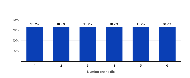
The uniform distribution describes a situation where all outcomes are equally likely. Rolling a die has six outcomes (1 to 6), and each has the same probability: 1 out of 6, or about 16.7%.

You can show a discrete distribution as a histogram: the possible values of the random variable go on the x-axis, and the probability of each value goes on the y-axis. For a uniform distribution every bar has the same height.

Histogram of a single die roll: six bars of equal height, each 16.7 percent — Chart 1 Every outcome of a single die roll has the same probability, so all bars are equally tall.

Where it is used

Data professionals often use the uniform distribution as a building block for more complex methods, such as Monte Carlo simulations. In a business setting, think of randomly assigning customers to one of several test groups: each group is equally likely. The uniform distribution also exists for continuous variables, not only discrete ones.

Bernoulli distribution

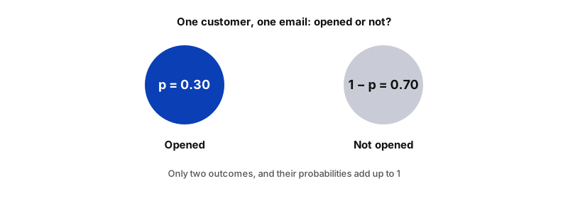
The Bernoulli distribution models a single trial with only two possible outcomes: success or failure. The two outcomes cannot happen at the same time. If the probability of success is p, the probability of failure is 1 − p.

A classic example is a single coin toss. In business data, it is a single customer who either opens a marketing email or does not. If 30% of customers open it, then p = 0.30 for success and 1 − p = 0.70 for failure.

Bernoulli distribution of one email: opened with probability 0.30, not opened with probability 0.70 — Chart 2 One trial, two outcomes. The probabilities p and 1 − p always add up to 1.

Success is just a label

"Success" and "failure" are labels chosen for convenience. For a coin toss you could call heads the success or tails the success, depending on what your analysis needs. In a fraud model, the "success" is usually the event you are trying to detect, such as a fraudulent transaction.

Binomial distribution

The binomial distribution is the Bernoulli distribution repeated. It models the number of successes in a fixed number of independent trials. The only difference is that Bernoulli covers one trial, while the binomial covers n trials. The process behind it is called a binomial experiment, which has four attributes:

Repeated trials. The experiment consists of a fixed number of trials.
Two outcomes. Each trial has only two possible outcomes: success or failure.
Same probability. The probability of success is the same for every trial.
Independence. Each trial is independent, so one result does not affect any other.

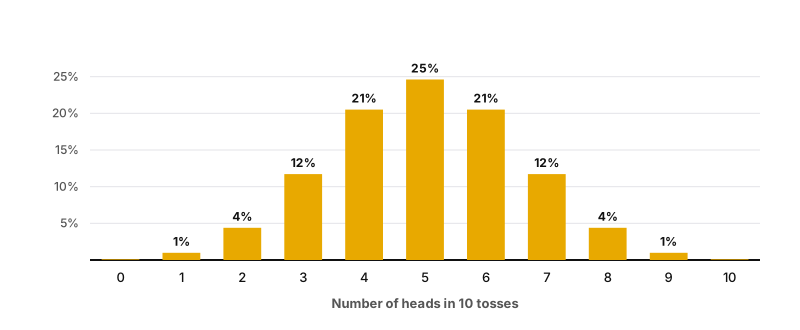
Tossing a coin 10 times in a row is a binomial experiment: there are 10 trials, each toss gives heads or tails, the probability of heads is 50% every time, and one toss does not influence the next. The histogram shows the number of heads on the x-axis and the probability of each result on the y-axis. The most likely result is 5 heads, at about 24.6%, and the bars fall away on both sides.

Binomial distribution of 10 coin tosses: bars peak at 5 heads with about 25 percent — Chart 3 Number of heads in 10 coin tosses. The shape is symmetric because the probability of heads is 50%.

Data professionals use the binomial distribution to model, for example, the probability that:

a new medication causes side effects,
a credit card transaction is fraudulent,
a stock price rises in value,
a customer who received an offer makes a purchase.

In machine learning, the binomial idea is also behind classification: an algorithm can be trained to decide whether a digital image shows a specific animal, like a cat or a dog, or not.

Poisson distribution

The Poisson distribution models the number of events that occur in a fixed period of time. It can also describe events in a fixed space, such as a distance, an area or a volume, but here we focus on time. A Poisson experiment has three attributes:

Countable. The number of events can be counted.
Known average. The mean number of events per time period is known.
Independence. Each event is independent of the others.

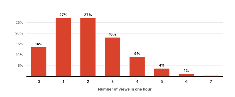
Imagine you publish content on a website that averages two views per hour. You want to know how likely it is to get a certain number of views in a given hour. This fits a Poisson experiment: views can be counted, the average of two per hour is known, and one person viewing the site does not affect whether another one does.

On the histogram, the x-axis shows the number of views per hour and the y-axis shows the probability. The tallest bars are 1 and 2 views, at about 27% each. Getting no views at all in an hour has a probability of about 14%.

Poisson distribution with an average of 2 views per hour: the tallest bars are 1 and 2 views at about 27 percent — Chart 4 Website views per hour with an average of 2. The distribution leans to the right: high counts are possible but rare.

Data professionals use the Poisson distribution to model the number of:

calls per hour in a customer service call center,
customers per day in a shop,
thunderstorms per month in a city,
financial transactions per second at a bank.

Which distribution should I use?

A quick way to choose is to ask what you are counting.

Distribution	What it models	Business example
Uniform	All outcomes equally likely	Randomly assigning a customer to 1 of 4 test groups
Bernoulli	One trial, two outcomes	One customer opens the email or not
Binomial	Number of successes in n independent trials	How many of 100 customers open the email
Poisson	Number of events in a fixed interval, with a known average	Support calls per hour

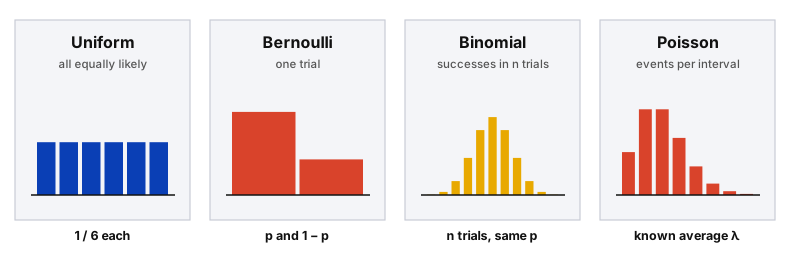
Four small bar charts: uniform with equal bars, Bernoulli with two bars, binomial with a bell-like shape, and Poisson leaning to the right — Chart 5 The four distributions side by side.

Binomial vs Poisson

Both count events, but the binomial has a fixed number of trials and a success probability (10 tosses, 50% each). The Poisson has no fixed number of trials, only an average rate per time period (2 views per hour).

Key takeaway

Identifying the distribution of your data is a key step in any analysis, and it helps you make informed predictions about future outcomes. Discrete distributions like the binomial and the Poisson are the ones you will meet most often as a data professional. Knowing the distribution of your data also helps you choose the statistical method or machine learning model that works best for your analysis.